# Clear environment
rm(list = ls(globalenv()))

# Load package
library(lidR)
library(sf)Area Based Approach
Relevant Resources
Overview
This code demonstrates an example of the area-based approach for LiDAR data. Basic usage involves computing mean and max height of points within 10x10 m pixels and visualizing the results. The code shows how to compute multiple metrics simultaneously and use predefined metric sets. Advanced usage introduces user-defined metrics for more specialized calculations.
Environment
Basic Usage
We’ll cover the basic usage of the lidR package to compute metrics from LiDAR data.
# Load LiDAR data, excluding withheld flag points
las <- readLAS(files = "data/MixedEucaNat_normalized.laz", select = "*",  filter = "-set_withheld_flag 0")
The pixel_metrics() function calculates structural metrics within a defined spatial resolution (res).
# Compute the mean height of points within 10x10 m pixels
hmean <- pixel_metrics(las = las, func = ~mean(Z), res = 10)
hmean
#> class       : SpatRaster
#> dimensions  : 15, 15, 1  (nrow, ncol, nlyr)
#> resolution  : 10, 10  (x, y)
#> extent      : 203830, 203980, 7358900, 7359050  (xmin, xmax, ymin, ymax)
#> coord. ref. : SIRGAS 2000 / UTM zone 23S (EPSG:31983)
#> source(s)   : memory
#> name        :           V1
#> min value   :  0.001065319
#> max value   : 17.730712824
plot(hmean, col = height.colors(50))![]()
# Compute the max height of points within 10x10 m pixels
hmax <- pixel_metrics(las = las, func = ~max(Z), res = 10)
hmax
#> class       : SpatRaster
#> dimensions  : 15, 15, 1  (nrow, ncol, nlyr)
#> resolution  : 10, 10  (x, y)
#> extent      : 203830, 203980, 7358900, 7359050  (xmin, xmax, ymin, ymax)
#> coord. ref. : SIRGAS 2000 / UTM zone 23S (EPSG:31983)
#> source(s)   : memory
#> name        :    V1
#> min value   :  0.75
#> max value   : 34.46
plot(hmax, col = height.colors(50))![]()
You can specify that multiple metrics should be calculated by housing them in a list().
# Compute several metrics at once using a list
metrics <- pixel_metrics(las = las, func = ~list(hmax = max(Z), hmean = mean(Z)), res = 10)
metrics
#> class       : SpatRaster
#> dimensions  : 15, 15, 2  (nrow, ncol, nlyr)
#> resolution  : 10, 10  (x, y)
#> extent      : 203830, 203980, 7358900, 7359050  (xmin, xmax, ymin, ymax)
#> coord. ref. : SIRGAS 2000 / UTM zone 23S (EPSG:31983)
#> source(s)   : memory
#> names       :  hmax,        hmean
#> min values  :  0.75,  0.001065319
#> max values  : 34.46, 17.730712824
plot(metrics, col = height.colors(50))![]()
Pre-defined metric sets are available, such as .stdmetrics_z. See more here.
# Simplify computing metrics with predefined sets of metrics
metrics <- pixel_metrics(las = las, func = .stdmetrics_z, res = 10)
metrics
#> class       : SpatRaster
#> dimensions  : 15, 15, 36  (nrow, ncol, nlyr)
#> resolution  : 10, 10  (x, y)
#> extent      : 203830, 203980, 7358900, 7359050  (xmin, xmax, ymin, ymax)
#> coord. ref. : SIRGAS 2000 / UTM zone 23S (EPSG:31983)
#> source(s)   : memory
#> names       :  zmax,        zmean,         zsd,     zskew,       zkurt,    zentropy, ...
#> min values  :  0.75,  0.001065319,  0.02499118, -1.860858,    1.127885, 0.005277377, ...
#> max values  : 34.46, 17.730712824, 12.95950270, 41.207184, 1738.774391, 0.955121240, ...
plot(metrics, col = height.colors(50))![]()
# Plot a specific metric from the predefined set
plot(metrics, "zsd", col = height.colors(50))![]()
Advanced Usage with User-Defined Metrics
lidR provides flexibility for users to define custom metrics. Check out 3rd party packages like lidRmetrics for suites of metrics.
We can also create our own user-defined metric functions. This demonstrates the flexibility of the lidR package!
# Generate a user-defined function to compute biomass
f <- function(z, dbh) { 0.2*(mean(z)^3) + 0.8*quantile(z, probs = 0.9)*dbh^2 }

# Compute grid metrics for the user-defined function
X <- pixel_metrics(las = las, func = ~f(z = Z, dbh = 0.4), res = 10)

# Compute grid metrics using the same function, using first returns only
X <- pixel_metrics(las = filter_first(las), func = ~f(z = Z, dbh = 0.4), res = 10)

# Visualize the output
plot(X, col = height.colors(50))![]()
Case Study: Vertical Complexity Index (VCI)
Let’s create a user-defined function for a more sophisticated metric. Vertical Complexity Index, or VCI, assesses the “evenness” of the vertical canopy structure using the same information theory as Simpson’s Evenness Index. As the vertical distribution of points becomes more unimodal, VCI approaches one; as the distribution of points becomes multimodal or skewed, VCI approaches zero. This metric was developed by Van Ewijk (2015).
\[VCI = (-\sum_{i=1}^{HB}[p_{i}*ln(p_{i}])/ln(HB)\]
Steps:
- Divide the vertical range of the pixel into a number of height bins
HB. - Compute the proportion
p_iof total returns in each height bini. - For each height bin
i, multiply the proportion of returnsp_iby the natural log of the proportion of returnsln(p_i). - Take the sum of these products and multiply by -1.
- Divide the negative sum by the natural log of the number of height bins
ln(HB).
# Build our function
f_vci <- function(z, bin.size) {
## Step 1: Specify the breakpoints for the bins.
brks <- seq(0, ceiling(max(z)), by = bin.size)
brks
## Step 2: Get the number of returns in each bin and divide by the total number of returns to get the proportion
z_counts <- hist(z, breaks = brks, plot = F)$counts
z_counts
z_prop <- z_counts / sum(z_counts)
z_prop
## Step 3: Compute the product of the proportion and the log of proportion using some simple vector algebra
z_products <- z_prop * log(z_prop)
z_products
## Step 4: Take the sum of the products and multiply by -1
sum_term <- sum(z_products) * -1
sum_term
## Step 5: Divide the negative sum by the natural log of the number of height bins
hb <- length(brks) - 1
hb
vci <- sum_term/log(hb)
vci
## Return the VCI
return(vci)
}

# Try out our new formula
VCI <- pixel_metrics(las = las, res = 10, func = ~f_vci(z = Z, bin.size = 1))
plot(VCI)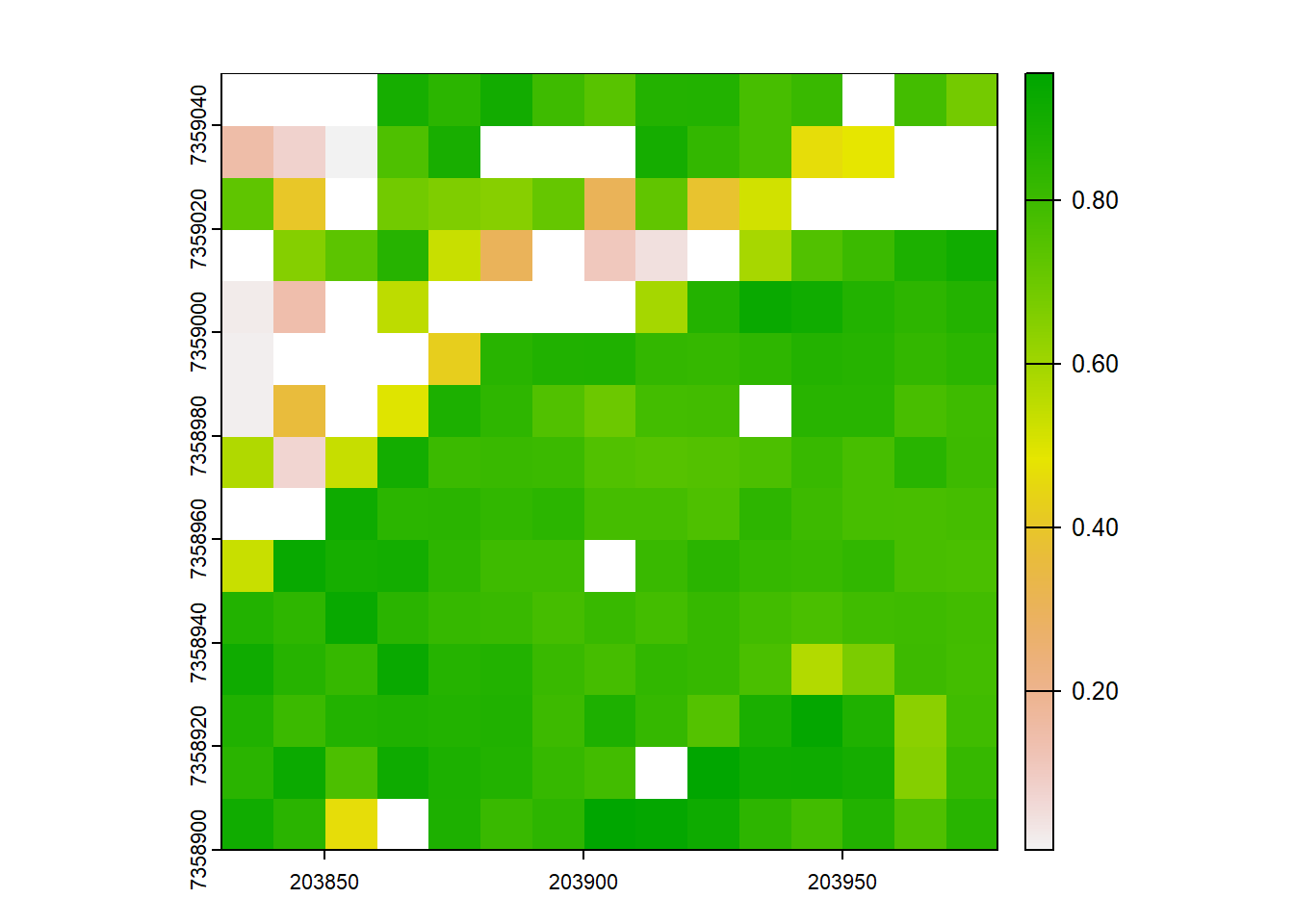
# Try it again, but use only first returns
VCI <- pixel_metrics(las = filter_first(las), res = 10, func = ~f_vci(Z))
plot(VCI)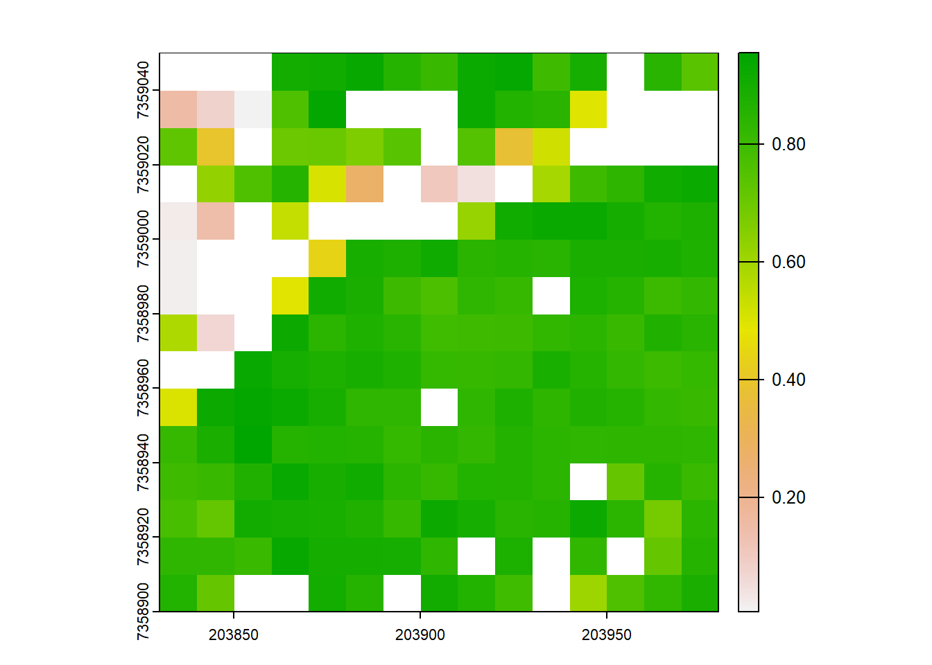
Exercises and Questions
Using:
las <- readLAS("data/MixedEucaNat_normalized.laz", select = "*", filter = "-set_withheld_flag 0")E1.
Using only first returns, calculate the difference between the mean height and 75th height percentile at a 10 m resolution. Plot both the raster output and the original point cloud and compare the trees where the difference is higher vs lower. What differences do you notice?
E2.
Map the density of ground returns at a 5 m resolution with pixel_metrics(filter = ~Classification == LASGROUND).
E3.
Map pixels that are flat (planar) using stdshapemetrics. These could indicate potential roads.
Conclusion
In this tutorial, we covered basic usage of the lidR package for computing mean and max heights within grid cells and using predefined sets of metrics. Additionally, we explored the advanced usage with the ability to define user-specific metrics for grid computation.